The sizzling steam engine

Steam engines are now museum pieces, but before the advent of the internal combustion engine and electric motors, they were the workhorses of industry, powering everything from water pumping stations to ships, dockside cranes, cotton mills and all sorts of factory machinery. By building one out of Lego, not only will you learn a lot about mechanics, but you will also gain a fascinating insight into control theory, one of the most important disciplines in 21st century engineering. To see the connection, read on!

Some annotated photographs
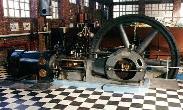	The principal components of a steam engine are the cylinder (left), which is connected via a connecting rod and crank (centre) to a large flywheel (right). In the simplest engines, high pressure steam flows into the cylinder to push the piston out and start the flywheel rotating. During the second half of the cycle, the flywheel pushes the piston back in and the steam leaves the cylinder through an exhaust valve. So mechanical power is applied during only half the cycle (when the steam expands inside the cylinder), but the flywheel smooths things out and keeps everything rotating during the second half of the cycle. Above the connecting rod is a strange looking contraption with two balls called a Watt governor, after James Watt, who used it in his early beam engines. Watt did not, however, invent the governor: similar devices were employed in wind and water mills many years earlier. The Watt governor is the link between the steam engine and control theory, and it is all to do with trying to keep the engine going at a constant speed when the mechanical load changes.
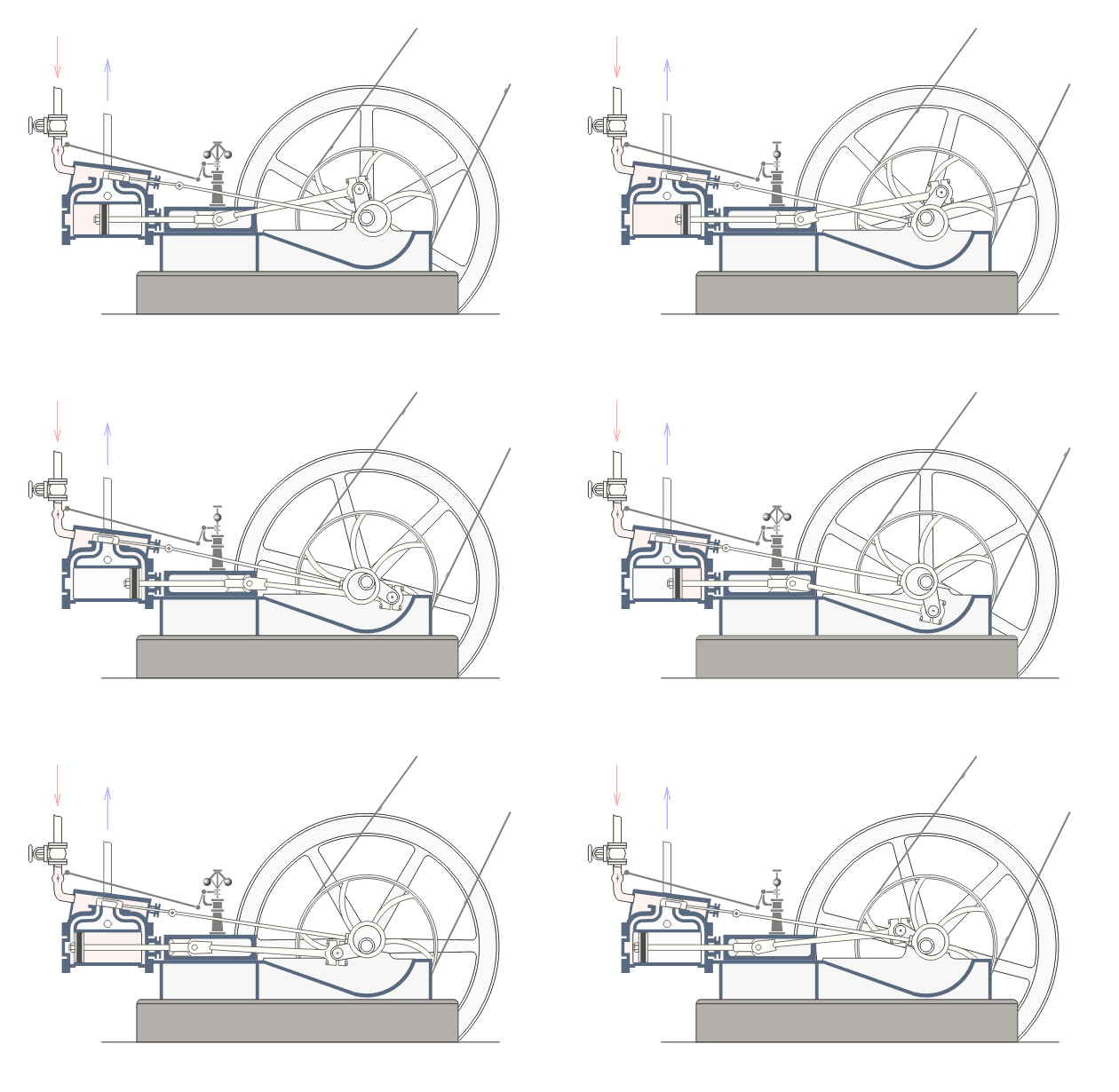	Typically, steam engines would have powered many machines at once. The drive from the slowly rotating flywheel would be geared up and fed to an overhead shaft running the length of the factory roof. From here, belts would drop down to individual machines, be they lathes, drills or looms. To start the machine, the operator would slip the belt onto a pulley and the machine would spin up. When this happens, though, there is more mechanical load on the steam engine, which needs to work harder (more steam!) to keep the drive shaft rotating at the same speed. The Watt governor makes this speed control automatic. It is a centrifugal device: the faster it rotates, the higher the spinning wheels climb on their axle, just like spinning a weight on a string above your head. Take a look at this nice simulation. Now turn your attention again to the animation on the left, and notice the mechanical linkage between the governor and the steam input valve on the cylinder. So, as the engine speeds up, the balls climb and the valve closes, reducing the amount of steam fed to the cylinder and consequently the force with which the piston is driven. Conversely, if the engine is running too slowly (e.g. if somebody has just connected another machine), the balls fall and the valve opens, increasing the force with which the piston is driven. This sort of proportional control aims to stabilize the engine speed at some set point. Sometimes, proportional control is perfectly adequate, but more often we need to draw on more advanced forms of control theory, as we shall shortly see. Note that the example on the left is a double-acting steam engine, with the piston being powered in both directions. We, though, will be building the simpler, single-acting variant. [Animation, left, reproduced with permission from Wikipedia]
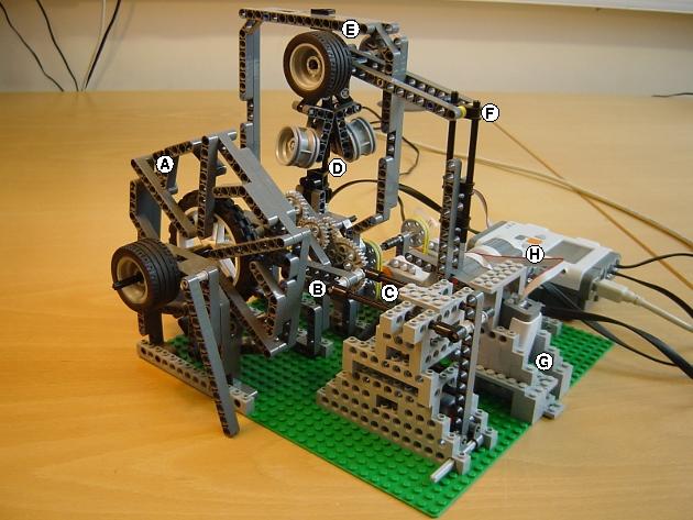	Here is the Lego steam engine at rest. At the front is the flywheel (A) connected via a connecting rod (B) to the piston (C). Above the Watt governor (D) are some wheels (E) which add inertia to the governor mechanism. By adding or removing tyres, it is possible to tune how much the governor rises or falls in response to speed variations. The governor is connected through a mechanical linkage (F) to a light sensor (G) which mimics the steam valve. As the governor rises, the light sensor is tilted towards the vertical and its output (it is pointing at a shiny Lego plate) increases. The light sensor reading is used by the Python program to control the flywheel speed. Finally, in lieu of real steam power, there are a couple of Lego motors (H) to drive the flywheel.
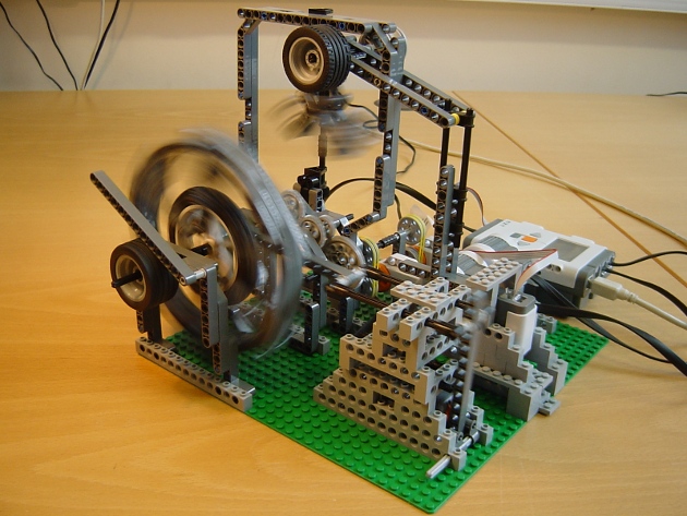	Here is the engine running at speed. Compared with the previous photograph, note how the governor has risen and the light sensor has tilted towards the vertical. Its reading has increased from a quiescent value of 300 to around 450. We could have mounted the light sensor up near the governor, pointing directly at the tyres, but its present position, hidden away between two little walls, has the advantage of being shielded from changes in the ambient light level. Note also the friction brake (the dark grey beam) applied to the leftmost tyre on the flywheel axle. This applies mechanical load, just like somebody attaching another machine in a factory. We can flip the brake on and off, and check that the motor power is adjusted automatically to keep the flywheel running at the same speed. Here is a movie showing the brake being engaged and then disengaged, and the engine automatically adjusting power to compensate.
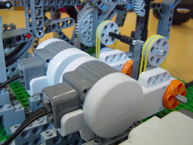	This photograph shows a close-up of the motors. We need two motors because the flywheel has a fair amount of inertia. The motor axles are not connected together directly: this would be a very bad idea, since no two motors are identical and they will not run at precisely the same speed! Instead, they both drive a common axle through elastic belts and pulleys. This also makes start-up less problematic: the high inertia might stall a stationary motor, but with this design the motors can spin up while the belts slip on the pulleys.
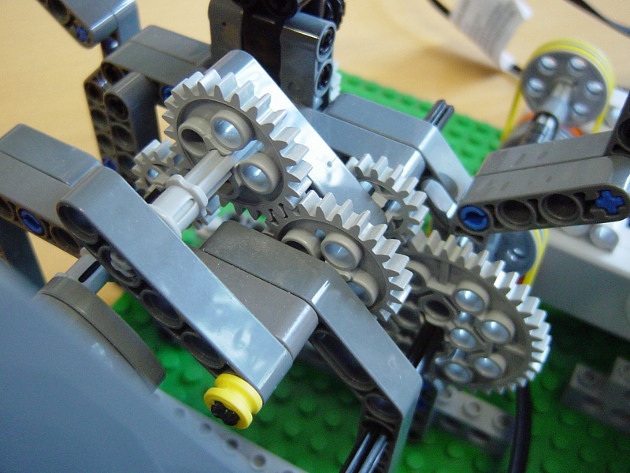	This is the gear train between the motor drive shaft (40-tooth gear, bottom right) and the flywheel axle (16-tooth gear, far left). The flywheel rotates faster than the motors, the ratio being (40/16) * (24/16) = 3.75. The second 24-tooth gear is an idler and does not affect the gear ratios: see the gears tutorial if you do not understand why. In this instance, though, the idler gear is mounted on a pivot that allows it to engage only when it is being driven clockwise from the motor side. It cannot transmit torque the other way, from the flywheel to the motor: all that happens is that the 16-tooth gear rotates and the 24-tooth idler jumps on its pivot. This is just like the ratchet on a bicycle freewheel: when you are pedaling it transmits torque to the wheel, but when you stop pedaling it does not allow the wheel to turn the pedals.
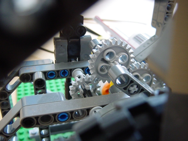	Here is another view of the ratchet idler gear, showing the pivot in action. This is what happens when the flywheel axle (with the 16-tooth gear) tries to drive the idler gear. As the 16-tooth gear rotates anticlockwise, it does not mesh with the idler gear but instead just pushes it up on its pivot: note how the teeth are not meshed in the photograph! We need this ratchet in our design because the motors imitate a single-acting cylinder and drive the flywheel for only half the cycle. For the other half of the cycle, the flywheel will continue to rotate freely with the ratchet jumping and no interference from the stationary motors. Then the motors will spin up again, torque will be transmitted through the idler, and the cycle starts over. It is just like you pedaling on your bicycle for one second, then freewheeling for one second, then pedaling again, imitating what a single-acting steam piston would do: push, vent steam, push, vent steam.
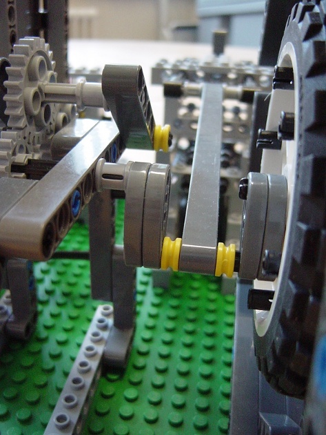	This view shows the 16-tooth gear (left, this time meshed with the ratchet idler) and how it is connected to the flywheel through a crank. A long connecting rod is attached to the bottom of the crank at its near end and the piston at its far end.
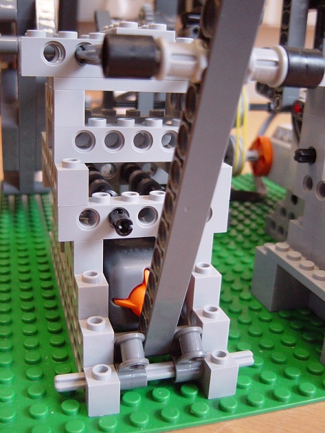	Here is the view from the far side of the piston, showing the touch sensor that is pressed and released by the upright beam once per cycle. We need this sensor so we can measure the cycle period, by timing the interval between consecutive presses. We can then power the motor for just half of this time, thereby simulating a single-acting cylinder. You can just about see how the touch sensor is suspended from two parallel axles on friction connectors. This makes it really easy to adjust its position: just slide it up and down the axles.
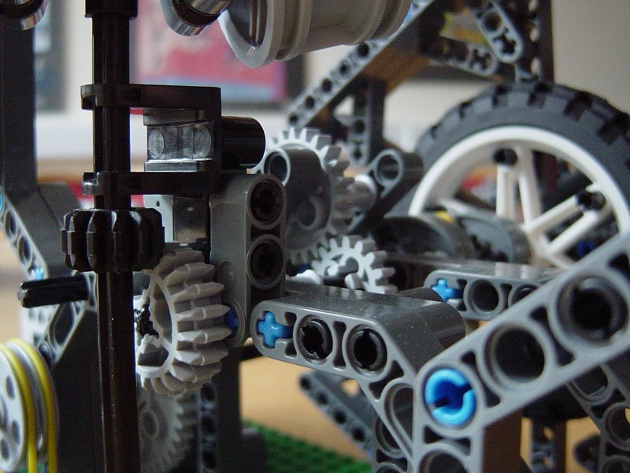	Here is the flywheel axle viewed from the other side, showing the bevel gears used to drive the Watt governor's vertical axle. As well as turning the corner, the bevel gears also gear up in the ratio 20:12, so the governor spins faster than the flywheel.
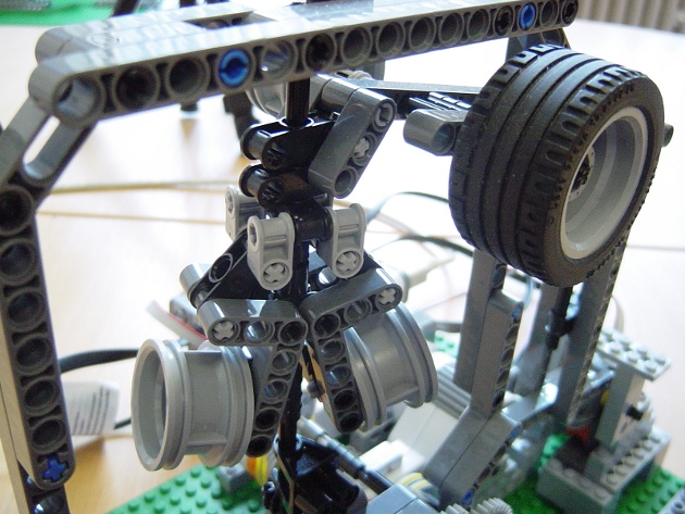	A close-up view of the Watt governor at its lowest position ...
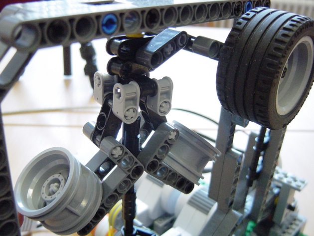	... and at its highest position. This is tricky to design, but detailed building instructions are available here. The governor pushes up on a lever mechanism, whose inertia can be adjusted by adding or removing tyres from the wheels (top right).
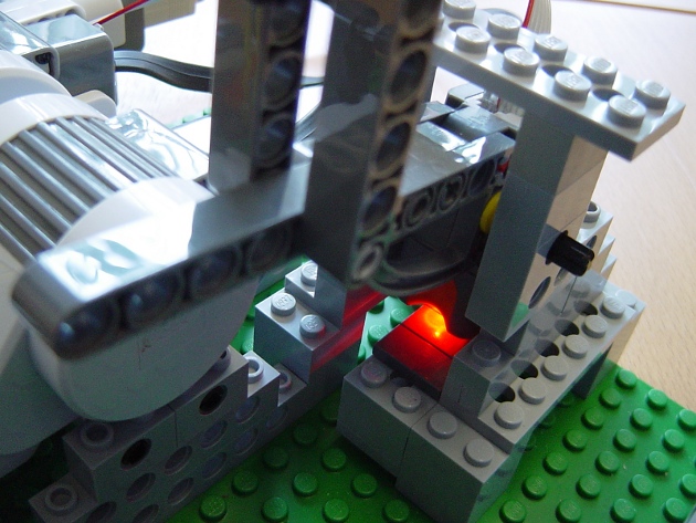	The other end of the lever mechanism tilts the light sensor inside its shaded enclosure. Here is a photograph taken at low speed: governor low, this end of the lever high, light sensor tilted away from the vertical, light sensor reading relatively low since the light is not reflected back into the photodetector.
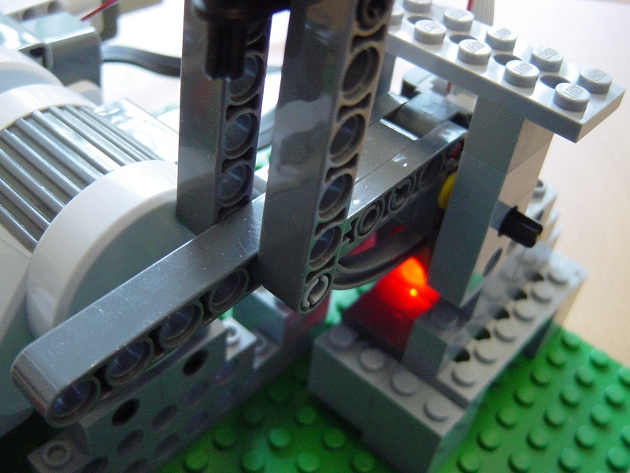	And here is what happens at high speed: governor high, this end of the lever low, light sensor vertical, light sensor reading relatively high since the light is reflected straight back into the photodetector.
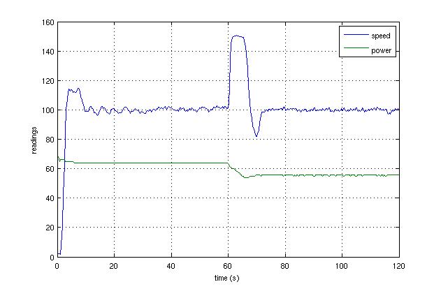	Finally, we should discuss the control theory that tells us how to set the motor power. We supply Python software (see below) that implements a generic proportional-integral-derivative (PID) controller: motor power = bias + proportional_gain * speed_error + integral_gain * integrated_speed_error + derivative_gain * rate_of_change_of_speed_error. So the motor power depends on the current speed error, the accumulated (integrated) speed error over time, and the rate of change of the speed error. The three gain terms are constants which need to be tuned for optimal performance. There is also a bias term, since the motor requires a certain amount of power even when there is no error! The graph on the left shows results of a two minute run of the steam engine with a target "speed" of 100 and nicely tuned gain terms. The "speed" trace is the difference between the light sensor reading and its quiescent value, so 0 when the engine is at rest. The friction brake was initially engaged, but released after one minute. Note how the engine initially speeds up as the mechanical load is reduced, but quite quickly settles back down to 100, albeit with a little overshoot. The motor power decreased, automatically, from around 65% to around 55% when the brake was disengaged.
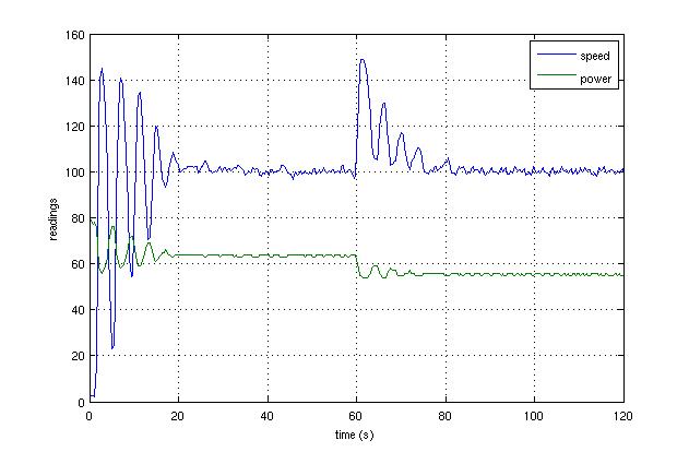	Here is a second run of the same experiment, this time with less well tuned parameters. The engine takes longer to settle when it is switched on and subsequently disturbed, with more overshoots. For now, you should just experiment with different gains and try to get a feel for what the various terms do. You will be introduced to formal control theory in your second year at Cambridge. If you cannot wait, the Wikipedia article on PID control is fairly comprehensible!

Here are some points to bear in mind if you decide to build your own steam engine.

• The Python program to run the engine is relatively subtle, which is why we are supplying it here. Connect your two motors to motor ports A and B, your light sensor to sensor port 1 and your touch sensor to sensor port 2. Towards the top of the program, you will find several variables that you will need to tweak. run_time is the length of the simulation in seconds, target_speed is what it says, and power_fraction is the fraction of the cycle that is powered by the motors (0.5 to simulate a single-acting cylinder). Then there are the four control parameters, corresponding to the four constants in the PID control law described above. The program starts off by spinning the motors continuously, just to get things moving. It then measures the cycle time using the touch sensor, and subsequently applies power to the motors only for the appropriate fraction of the cycle. The cycle time is continuously re-estimated as the engine runs, and the motor power is adjusted, according to the PID law, once per cycle. At the end of the run, it produces speed/power graphs, just like the ones above.

• If you are interested in control theory but think the mechanical subtleties of the engine might be a little too ambitious, here's a simplification. Do away with the piston, touch sensor and ratchet. You will no longer be able to simulate a single-acting cylinder (since there is no way to measure the cycle time), but you can run the motors continuously to imitate a double-acting engine, like in the animation near the top of this page. The supplied software will cope: just set power_fraction = 1.0, the program then assumes there is no touch sensor and powers the motors continuously.

• Look closely at your belt drives and the pulleys they are connected to. Run the motors continuously (set power_fraction=1.0) and observe how the lower (driver) pulleys rotate slightly faster than the upper (driven) ones. Why?

• Now try running with one motor: this is easily done by removing the elastic bands from one of the pulley sets. How does this effect the performance of your engine? Why?

• Experiment with different values of the control parameters while flipping the friction brake on and off. You can adjust the braking force by adding or removing pieces from the beam. Observe how there is generally a trade-off between speed of response and stability. Notice how some parameter combinations make the system unstable, with the engine never settling at the required speed. While you might have some intuition as to why this might be, you will need to wait for the second year control course before you can analyse these phenomena quantitatively.

The sizzling steam engine was designed and built by Paul McMahon in March 2010.