Stradview can be used to fit a shape model to thresholded data. This tutorial walks through the process of fitting a model of the otic capsule to pseudo-clinical multidetector CT data.
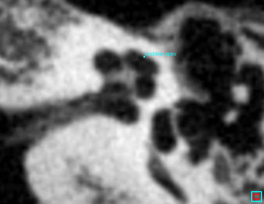
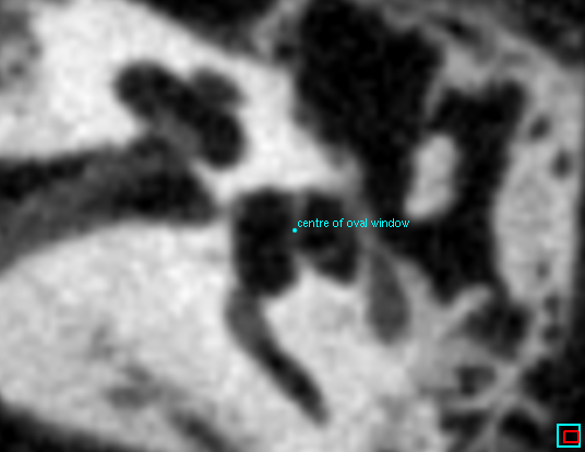
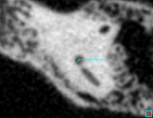
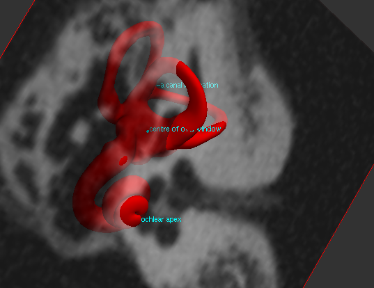
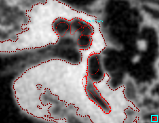
After opening the CT data file, the next step is to load the appropriate shape model (which can just be a simple surface mesh) using the Load button in the fit shape model task. In this case, we have loaded the canonical_otic_capsule.ply file which is distributed with Stradview. Next, we locate the three landmarks by clicking in the top-left canvas with the landmark tool. For the otic capsule model, Stradview prompts the user to locate the cochlear apex, the centre of the oval window and the posterior-anterior canal bifurcation.
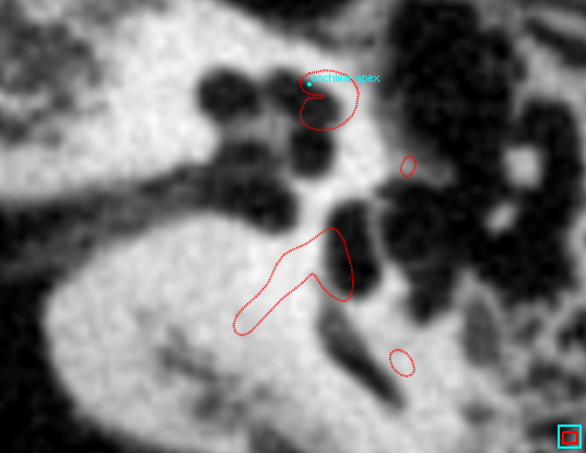
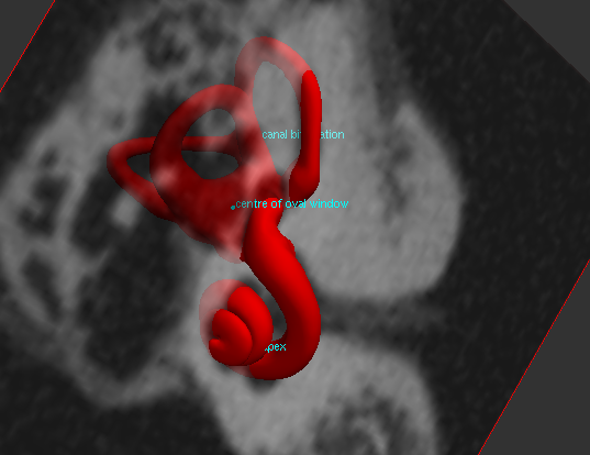
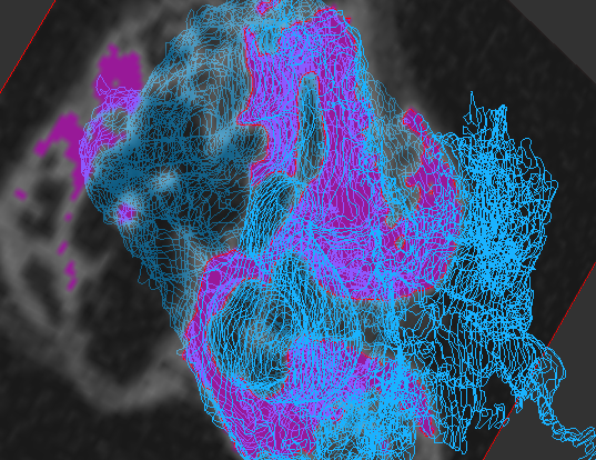
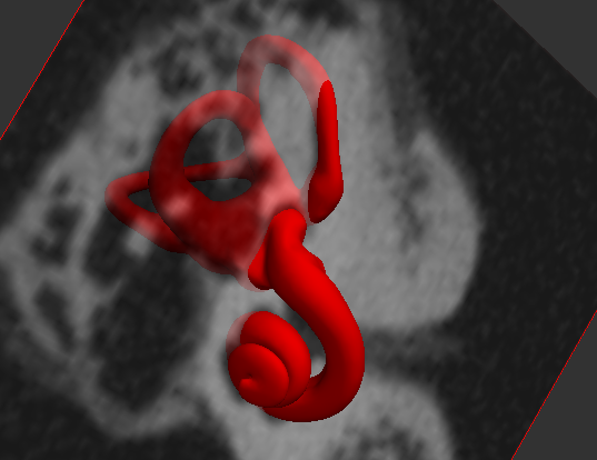
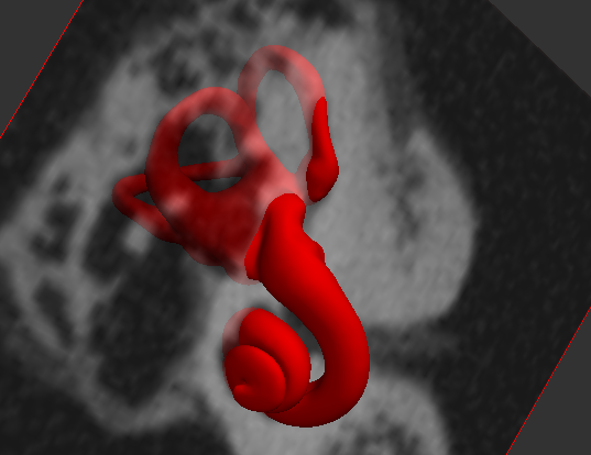
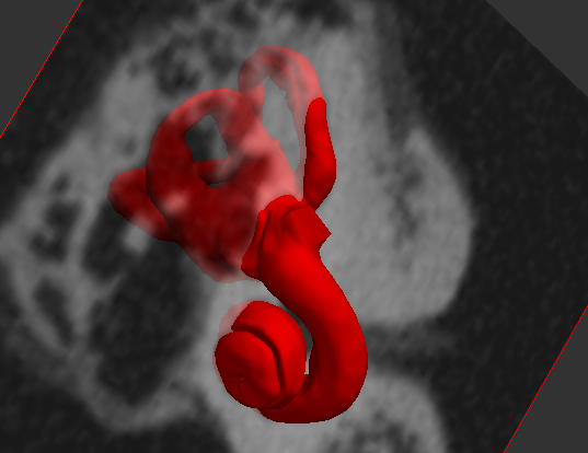
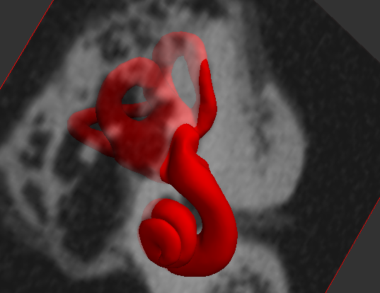
We can now press the Fit to landmarks button. This fits the shape model to the three landmarks, up to an unknown reflection in the plane defined by the landmarks. The left two images below show a fit with the incorrect chirality. The failure is obvious from a cursory inspection of the way the model intersects the CT data. We correct the fit by pressing the Fit to landmarks button a second time, which reflects the model in the landmarks' plane, as shown in the right two images below.
For loaded surfaces without landmarks, this process must be completed manually by using the control key while clicking and dragging in the 3D window.
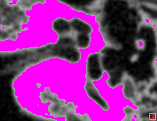
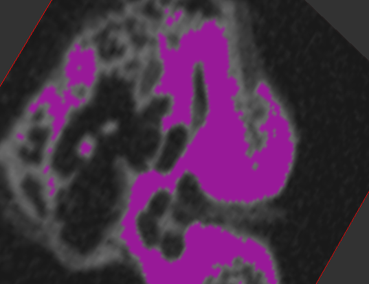
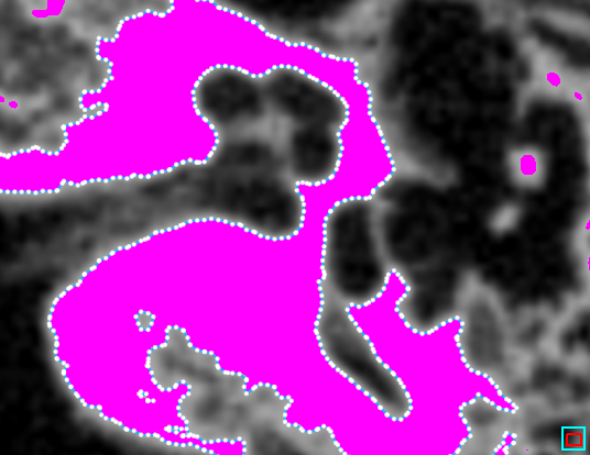
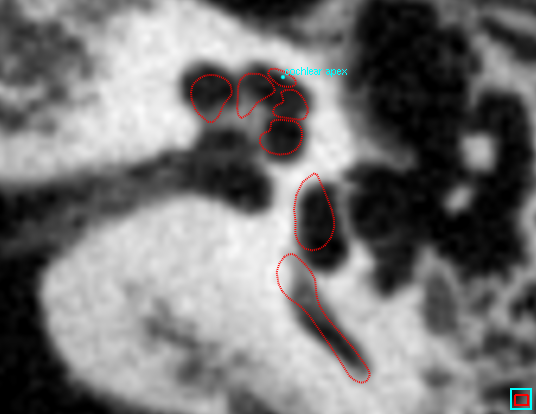
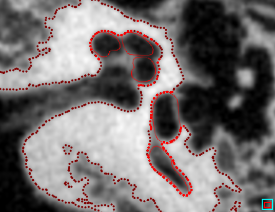
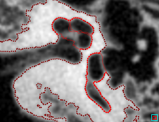
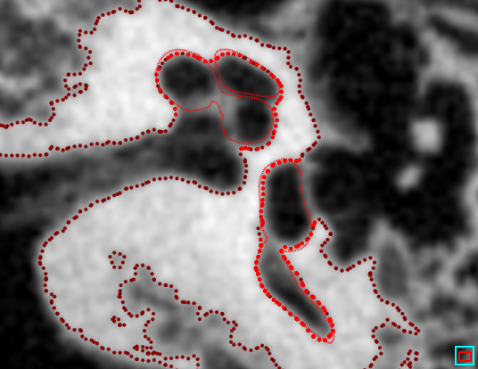
We now map the segmentation vertices back into the fit shape model task. After selecting the appropriate object to map the points from, we press the Map points button. The segmentation vertices are now shown as dark red dots. Those which are matched to a vertex of the shape model are shown in bright red. In the left image below, there are many dark red dots which should be bright. This error has occurred because Stradview considers surface normals when matching points, and in this instance is attempting to match outward pointing normals from the magenta region to outward pointing normals on the shape model, whereas we should be using inward pointing normals from the magenta region. So we select the in option for Match inside/outside and press the Map points button again, producing the image on the right.

If necessary, the inside/outside normal check can be disabled by selecting the both option for Match inside/outside. There is also the option to manually add and delete red points using the landmark and erase tools, but we shall proceed without manual intervention in this example.
Next, we refine the model fit by pressing the Start registration button. The images below show the results of 50 iterations with the Nonrigid flexibility slider set to 0. This is the best fit using just a rigid body transformation plus isotropic scaling.

Finally, we add some nonrigid deformation. The images below show the results of 50 iterations of locally affine deformation (LAD) with the Nonrigid flexibility slider set to 1. Just a little nonrigid flexibility implies a high degree of regularization, with smoothness favoured over a close fit to the red dots.
As shown below, more flexibility/less regularization produces obviously incorrect fits with this low resolution, noisy data. The problem is that there are no red dots to constrain the fit at the medial wall of the cochlea or the round and oval windows, since the simple threshold cannot pick out the boundaries in these regions.
By selecting SSM instead of LAD, the nonrigid deformation is guided by a statistical shape model instead of the locally affine deformation. A good fit results in this case (see below), since we are fitting to one of the 18 specimens used to train the SSM, i.e. we are cheating! With unseen specimens and an SSM trained on only 18 exemplars, we have found that the LAD approach works better. Some of Stradview's other SSMs are trained on much larger numbers of specimens, and are therefore potentially more useful.
With the model fitted to our satisfaction, we can now press the Save surface button to save the surface as a .ply or .wrl file, or use the Map back to object controls to generate a set of segmentation contours from the fitted surface, for use in the draw task.