Cortical Bone Mapping (CBM) is a technique for making surface-based measurements of the properties of a laminar object from a 3D data set. Usually this is a bone, from CT data, and the properties are thickness, mass, inner (trabecular) density etc. However, the technique can also be used for instance on the space between objects (Joint Space Mapping, JSM, or cartilage in MRI data).
The method follows three stages. First, the object of interest (for instance a bone) needs to be approximately segmentated to create its outer surface. Then various measurements are made of the data, at locations guided by this surface. Lastly, these measurements can be smoothed and visualised, new, more accurate, surfaces created, or used to sample the (eg. parametric MRI) data from between the surfaces.
Creating a surface for the object you wish to measure can be done in Stradview by following the relevant How-To, or alternatively loaded in from an external package. In any case, it should only follow the outer surface, not the inner. When deciding what resolution surface to use, bear in mind that the CBM procedure will make a measurement at each vertex on the surface (i.e. at the corner of each of the triangles). You should aim for enough measurements to cover any likely local variations, but not so many that any following analysis becomes more difficult. Regularised Marching Tetrahedra, implemented within Stradview, is particularly good at generating surfaces with very uniformly spaced vertices, ideal for this process.
CBM measurements will not be made over surface 'caps': the flat regions at either end of the surface. If your surface ends within the data set, make sure that 'triangulate over ends' is checked. Alternatively, if the surface is cut off by the end of the data, make sure that there is an outline on the last image, so that a flat cap will be created at this point.
If you only need to make CBM measurements over a small portion of the surface, then you can create a surface patch from this surface, move this patch to a new object, and then just make measurements over this new object. Patches are created by drawing on the surface. It is often easier to see where to draw by using the 'compounding' optionr to project the data onto this surface.
The approximate surface does not need to be exactly in the right place: for typical clinical CT data, it only needs to be within a couple of mm of the required surface, ideally outside rather than inside the outer cortex. It is more important that it is fairly smooth, so that the direction normal to the surface always goes through the outer surface nearly at a right angle. It is often better, for instance, to ignore local small features in the surface (for instance small divots in the cortex, or osteophytes on bone) at this stage.
Having defined the surface, measurements are made along lines through the data, using one of a variety of techniques, defined more fully in the 'thickness' task. You should set the line length to roughly three times the thickness of the thickest cortex you expect to see in the data. Having done this, position a typical line in the data by using the 'measure' tool, by clicking just outside the surface, then dragging outwards to adjust the orientation of this line. You should then see the data along this line plotted in blue on the lower visualisation window. If this data looks very noisy, you can increase the 'line width' from zero (the default). This will average together the data from several lines close to each measurement location. It is not usually necessary on clinical CT data, but may well be a good idea on noisy cone beam CT or very high resolution micro-CT data.
The various techniques are described in the 'thickness' task and in the corresponding papers. If you are using clinical CT data, it is probably best to start with 'CBM v2', or 'Endo CBM v2'. For high resolution micro-CT, you may get a good result with the (faster) 'auto-threshold' technique, and a larger value for 'line width'.
Some techniques, such as 'CBM v2' need an estimate of maximum cortical density and the in-plane and out-of-plane blur in the data. In that case, the 'estimate cortical density' button will be active (not greyed out). It is usually best to do this over all surfaces in the data (by leaving the 'current surface' set to 'none'). After running this process, the cortical density and blur values will be updated. If you save the file at this point, these values will be stored, so you don't have to repeat this process again if you re-load the data set. This cortical density value has a fairly significant impact on the measurements: so you should ensure that it is believable before continuing. If it is very low (for instance much less than 1000 HU for bone), then the thickness measurements will probably be over-estimates.
Now select the surface you are interested in and press 'map over current' to run CBM on that surface.
It is also possible to measure the distances between two surfaces using 'compare current to alternate'. Such measurements can either be the distance to the closest point, or measured in the direction of the surface normal at each point. If 'alternate' is set to the same surface as 'current', this will measure the distance through the object. So if you have manually segmented both the outer and inner cortical surfaces, the gap between them can be measured using this technique. As well as measuring distance, this approach will also sample the underlying data between the surfaces, then store the average values as the 'density' at each of the surface locations.
Measuring the distance through the object, as above, before running CBM, can also be used to detect incorrect measurements (see below), particularly useful if you are interested in the trabecular density.
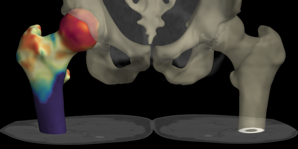
The CBM process makes several measurements simultaneously. In order to visualise these, select the appropriate measurement in the 'colour with' option, and ensure that the various range sliders below this allow you to see the variation in this data in the 3D window.
The individual measurements are likely to be noisy, might need outlier rejection and will probably need smoothing. Initially set the 'smoothing' slider to zero, so you can see all the original measurements. The coloured surface will probably look slightly speckled (occasional erroneous measurements) and have patches of gray (occasional failed measurements). You can adjust the two outlier sliders, 'reject angle above' and 'reject offset above' to affect this. As these sliders are altered, you will see more or less of the data marked as 'failed' (gray). Pick values which leave all the valid data visible but remove any measurements which look incorrect. Visualising the 'offset' can also help in this process.
If you have also measured the distance through the object, then the 'reject_offset_above' slider is also used to control whether these measurements are compared to the CBM ones. What this allows you to detect is situations where the thickness measurement is actually of the whole object, i.e. two cortices very close together, or a single cortex with no trabecular compartment. In this scenario, the inner density measurement might actually be of the soft tissue or air outside of the bone. Using this comparison, it is possible to reject such values.
Having rejected any outliers, the 'smoothing' slider can be used to remove any remaining grey regions: set to one, this simply fills in such regions with their nearest values, but higher values also smooth the data, being careful to pay more attention to data which is known to have more accurate measurements. If you have very large regions of the surface over which no CBM measurements were possible, you may want to set 'fill missing data' to lower than 100% so that these grey regions are not entirely filled in.
If you just want to make spot checks on the surface, you can click on the surface using the 'measure' tool, and Stradview will show you the details at this point in the middle status bar at the bottom of the Stradview window.
After running CBM over a surface, the average results over the whole surface are displayed in the thickness visualisation page.
All the individual results can be stored with the 'save results for current' button. This stores the original (unsmoothed) results, in addition to the smoothed results for whatever is currently being displayed. It also stores a copy of the cortical surfaces, coloured in the same way as the current visualisation in the 3D window. So this data is sufficient if you just want to visualise the results with a 3D viewer, or if you want to perform Statistical Parametric Mapping (SPM) on the results after registering the data using wxRegSurf.
Alternatively, it is possible to create another object in Stradview which precisely defines the outer and/or inner cortical edges. This process is described elsewhere, in the help for 'create surface in alternate'. This makes use of the outlier rejection and smoothing described above, as well as testing for consistency in the actual location of the new outer cortical surface: hence this is the most accurate way to generate outer and inner cortical surfaces. Since this creates a new Stradview object, it can be exported to a 3D surface file in the same way as for any other object.
There are several situations in which this latter approach is the appropriate one. Firstly, for internal visualisation: creating such a surface, and then visualising the intersections of this surface with the data using the 'find' button on the draw task, is a good way to check the accuracy of these measurements. Secondly, this is the best way to generate a surface if the intention is to use it for improving the accuracy of a Finite Element Analysis (FEA) model. This is also the only case where the 'map direction' should be set to anything other than 'normal'. Setting this to 'optimal' (and re-running the CBM measurements) should minimise the number of overlapping triangles in the created inner surface.
Lastly, having created a new surface, it can be used to sample the underlying data between the outer and inner surface layers. Select the new surface as both the current and alternate, then use 'compare current to alternate' to update the measurements for this new surface. The new 'density' values will represent the average of the underlying data between the surfaces, which can be visualised or saved with the other CBM data.
The 'density' results from CBM are all output in the same units as the data, so for CT they are in Hounsfield Units (HU) and do not strictly correspond to density. Conversion of HU to density is possible by using a QCT phantom, which is either scanned with the patient or in a separate sequence. Stradview understands several of these phantoms and can generate the calibration which will transform HU values to mg/cc. This calibration is not applied internally to the CBM data: you would need to use the two parameters from this equation in external software to actually convert the 'density' values.