Ultrasonic elasticity imaging

A special topic in displacement tracking

Introduction

Ultrasound elasticity imaging (or ultrasound strain imaging, or ultrasound elastography) is a medical imaging model for the evaluation of the mechanical properties of tissue. This general paradiam embraces a wide range of different techniques, the principal distinguishing factors being how the stress is applied and how the tissue deformation is measured.
In our group, we focus on the quasistatic approach to ultrasound elasticity imaging, where tissue deformation is introduced by pressing on the probe. Two radio frequency (RF) ultrasound frames are acquired pre and post-deformation. Some indication of the tissue elasticity is provided by the axial strain, which is usually retrieved in two steps: displacement estimation, by matching pre-deformation RF data windows with post-deformation windows; and strain estimation, by differentiating the displacement field.

Displacement estimation

Exhaustive search

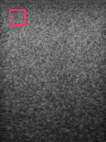
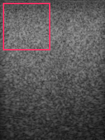
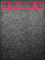
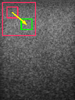
The simplest displacement estimation method is probably exhaustive search. A processing window is defined in the pre-deformation RF frame (Fig. 1(a)) and a search region is defined in the post-deformation RF frame (Fig. 1(b)). The standard cross-correlation similarity metric can be used to locate the best match of the processing window in the search region. The offset from the original window to the best matched window is the displacement of the window centre point (Fig. 1(c)). 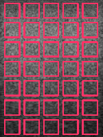Exhaustive search applies the same strategy to all windows in a RF frame to retrieve a displacement field (Fig. 1(d)).

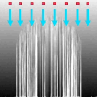
Displacement tracking

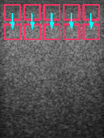
In the displacement tracking approach, only a few windows are searched within a big search region. For example in Fig. 2(a), windows in the top row are exhaustively searched. The search region of the 2nd row of windows are offset by the estimated displacement of the 1st row. This helps to reduce the search region size of the 2nd row of windows, since after position offset, a search region is roughly aligned with the corresponding window. In other words, displacement of the 2nd row of windows are “tracked” from the 1st row (Fig. 2(b)). Similarity, all subsequent windows keep tracking of the displacement from a previous row to build up a displacement field.

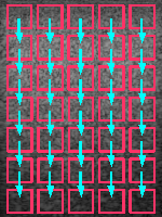
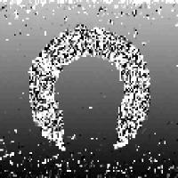
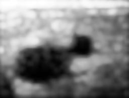
The displacement tracking approach is an improvement upon exhaustive search. It requires mush less processing time owing to the reduced search regions and implicitly imposes continuity constraint on the resultant displacement field. However, there is a special error-propagation problem associated with displacement tracking, as shown by Fig. 3. In Fig. 3(a), an arc region is masked by noise, where no valid displacement can be retrieved. If displacement tracking is performed from top to bottom, erroneous estimates start to accumulate in the arc and are passed on to all the regions below the arc (Fig. 3(b)). On the contrary, exhaustive search method can retrieve plausible displacement from the centre of the arc. As each window is processed independently, errors in the arc do not affect other regions (Fig. 3(c)).

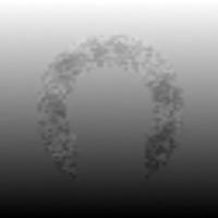
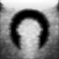
Quality-guided displacement tracking

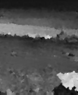
We recently developed a displacement estimation method called the quality-guided displacement tracking algorithm. It is capable of tracking around unreliable estimates and reducing error propagation. Figure 4(a) shows the axial displacement field of the same data set in Fig. 3(a) retrieved by the quality-guided displacement tracking algorithm. All regions except the arc have obtained plausible estimates. The post-alignment window-matching quality field is shown in Fig. 4(b). It is based on this quality map that the tracking path propagates. A video of the tracking progress is shown in Fig. 4(c), which can be played with Windows Media Player Plug-In. The tracking starts from several windows at different places (we call them seeds). It propagates the whole frame in a quality descending order, such that highly matched windows render their neighbours being processed earlier and poorly matched windows delay the processing of their neighbours. This strategy ensures that when tracking paths encounter the arc region, they are paused. Only after surrounding higher quality regions are finished, do the tracking paths enter the arc. In the arc estimation errors are inevitable but they will not affect other regions.

In Figure 5. a video illustration shows how exactly the quality-guided tracking algorithm works. Each cell on the video image represents a processing window. The number in a cell represents the matching quality of that window. At the initial stage, there are 3 seeds: red, green, and yellow; and they obtain displacement estimates and matching quality by exhaustive search. The tracking algorithm is responsible for deciding which is the next window to process. The governing rule is: the next window to processe is always a neighbour of a processed window that has the highest quality value. In this example, a neighbour (does not matter which neighbour) of the green window will be processed. After all neighbours of the green one are finished, the red window's quality becomes the global maximum. So a neighbour of the red will be processed and so on and so forth. Note, any neighbour of the yellow window will not be processed until the global maximum quality drops to 0.3 or until it is propagated from other seeds.

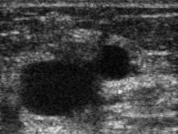
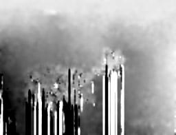
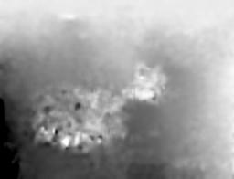
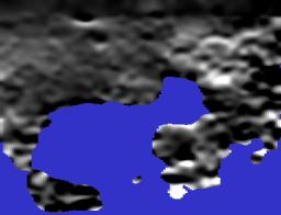
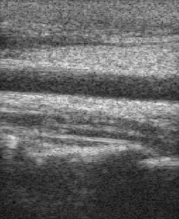
Figure 6 shows a breast scan that captures a cyst. Tissue displacement estimates inside the cyst are unreliable due to the lack of ultrasound wave scatters.

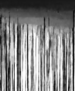
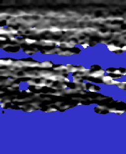
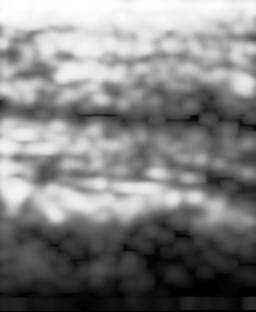
Figure 7 shows an artery scan. There are two challenges to displacement estimation. First, the artery was pulsating during the scan and created a discontinuous displacement field above and below the artery. Second, two high quality regions are separated by the artery and they must be independently tracked.

Last updated: January 2009