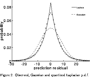


The samples in the prediction residual are now assumed to be uncorrelated and therefore may be coded independently. The problem of residual coding is therefore to find an appropriate form for the probability density function (p.d.f.) of the distribution of residual values so that they can be efficiently modelled. Figures 2 and 3 show the p.d.f. for the segmentally normalized residual of the polynomial predictor (the full linear predictor shows a similar p.d.f). The observed values are shown as open circles, the Gaussian p.d.f. is shown as dot-dash line and the Laplacian, or double sided exponential distribution is shown as a dashed line.
These figures demonstrate that the Laplacian p.d.f. fits the observed
distribution very well. This is convenient as there is a simple Huffman
code for this distribution [5][4][3]. To
form this code, a number is divided into a sign bit, the  th low order
bits and the the remaining high order bits. The high order bits are
treated as an integer and this number of 0's are transmitted followed by
a terminating 1. The
  low order bits then follow, as in the example
in table 1.
As with all Huffman codes, a whole number of bits are used per sample,
resulting in instantaneous decoding at the expense of introducing
quantization error in the p.d.f. This is illustrated with the points
marked '+' in figure 3. In the example,  giving a
minimum code length of 4. The error introduced by coding according to
the Laplacian p.d.f. instead of the true p.d.f. is only 0.004 bits per
sample, and the error introduced by using Huffman codes is only 0.12
bits per sample. These are small compared to a typical code length of 7
for 16 kHz speech corpora.
This Huffman code is also simple in that it may be encoded and decoded with a few logical operations. Thus the implementation need not employ a tree search for decoding, so reducing the computational and storage overheads associated with transmitting a more general p.d.f.
The optimal number of low order bits to be transmitted directly is linearly related to the variance of the signal. The Laplacian is defined as:

where  is the absolute value of
  and
and  is the variance of the
distribution. Taking the expectation of
  gives:

For optimal Huffman coding we need to find the number of low order bits,
 , such that such that half the samples lie in the range
  .
This ensures that the Huffman code is
  bits long with probability
0.5 and
  long with probability
  , which is
optimal.

Solving for  gives:
When polynomial filters are used  is obtained from
  using
equation 21. In the LPC implementation
  is derived
from
  which is obtained directly from the calculations for
predictor coefficients the using the autocorrelation method.


