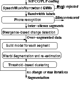
Figure 1: The segmenter
Abstract:
This paper describes the development of the Cambridge University RT-04
diarisation system, including details of the new segmentation and clustering
components.
The final system gives a diarisation error rate of
23.9% on the RT-04 evaluation data, a 34% relative improvement
over the RT-03s evaluation system. A further reduction down to 18.1% is
shown to be possible when using the segmentation algorithm alone.
The Rich Transcription diarisation evaluations[1, 2, 3] provide
a framework to analyse the performance of such speaker diarisation systems on
Broadcast News (BN) data.
A Diarisation Error Rate (DER) is defined which considers the
sum of the missed, false alarm and speaker-error
rates after an optimal one-to-one mapping of reference and hypothesis
speakers has been performed. (This mapping is necessary to associate
the 'relative' speaker labels such as 'spkr1' from the hypothesis to the
'true' speaker labels such as 'Ted Koppel' in the reference).
Cambridge University first built a complete diarisation system in
late 2002 and has participated in the diarisation evaluations since
then. This paper describes the development of the Cambridge University
diarisation system used in the Fall 2004 Rich Transcription
evaluation (RT-04)[3, 4].
The paper is structured as follows. Section 2 describes the diarisation system itself, sections 3 and 4 describe the data and scoring metrics used in the experiments, section 5 describes the development experiments, section 6 details the performance on the RT-04 evaluation data and plans for future work and conclusions are given in sections 7 and 8.
The speech signal is coded into MFCC, wideband (WB) PLP and narrowband
(NB) PLP coefficients every 10ms using a 25ms window.
The data is then divided into regions of WB speech (S),
speech with music (MS), NB speech (T) and music only (M) using a GMM
classifier incorporating an MLLR adaptation stage, based on 13 MFCC
features with first and second differentials.
The MS regions are relabelled as S and the M portions are discarded.
Wideband and narrowband data is subsequently treated independently.
A phone recogniser which has 45 context independent phone models per gender plus a silence model with a null language model is then run for each bandwidth. Silence portions longer than 1 second are discarded and the speech portions between these silences form the new segments. A change point detector then finds potential changes in audio characteristics within each segment. It uses a distance metric, dSD , based on the symmetric Kullback Leibler (symmetric divergence) distance [8]
![]()
These segments are then clustered into longer segments using an iterative segmentation-clustering algorithm for each bandwidth in the style of [6]. A model is built for each segment and the loss in likelihood when combining two segments is calculated from: [9]

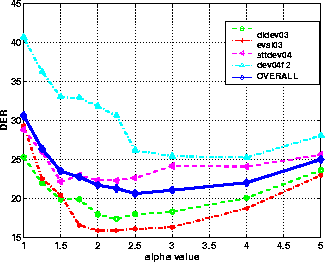
The clusterer uses the start and end times of the segments from the segmenter but makes no use of the speaker labels. The clustering is done bandwidth and gender dependently using a top-down approach. Each segment is represented by a single full correlation (not covariance) matrix of 13 static PLP (with c0) features. The arithmetic harmonic sphericity distance metric[12] is used to move the segments between the children nodes until convergence before using the BIC-based stopping criterion to determine whether a given split should occur. The standard BIC formulation, given in Equation 1, is used with the slight modification that a 'local' (number of frames in the parent cluster) rather than 'global' (number of frames in the whole show) value of N is used. L is the log likelihood of the data, #M is the number of free parameters and α is the tuning parameter (here 7.25).
After clustering, segments with the same cluster (speaker) label which are adjacent in time are merged. This does not affect the diarisation score in itself, but makes the segmentation clearer to a reader, and enables the iterative clustering scheme of section 5.6 to be easily implemented. This baseline clusterer is described in more detail in [11]. The RT-04 clusterer differed only in the way the segments were sorted before clustering, changing the initialisation. Section 5.4 has more details.
The didev03 set was the development data for the
spring RT-03 diarisation evaluation[2]
and the references were generated
using the process described in [13] using forced alignments
provided by the LDC with 0.3s of silence smoothing applied.
The eval03 and dev04f2 sets was the official
diarisation development data for the RT-04 diarisation evaluation,
and were generated in a similar way to the didev03 data
but used forced alignments from a LIMSI system and 0.5s silence smoothing.
The sttdev04 set was marked up manually
for speakers at Cambridge University and does not use the 0.5s smoothing
rule, but still offers a useful development set for diarisation experiments.
The key features of the development data sets are summarised in
Table 1.
| Name | didev03 | sttdev04 | eval03 | dev04f2 |
| Epoch | Oct-Dec 2000 | Jan 2001 | Feb 2001 | Nov/Dec 2003 |
| Spec. | RT-03s | CU | RT-04 | RT-04 |
| Alignment | LDC (words) | manual (spkrs) | LIMSI (words) | LIMSI (words) |
| Silence Smoothing | 0.3s | N/A | 0.5s | 0.5s |
The RT-04 diarisation evaluation data (eval04f) consisted of 12 shows broadcast in December 2003.
A 0.25s no-score region (collar) was used round reference segment boundaries during scoring and regions of overlapping speech in the reference were excluded from scoring.
Unlike the segmentation used in the Cambridge University RT-03 spring
(RT-03s) diarisation evaluation ([7]) it
produces putative speaker
labels as well as the start and end times and hypothesised bandwidth of
each segment. This enables a DER to be obtained after
the segmentation stage. However, since there is a subsequent clustering
stage in the diarisation system (which makes no use of the putative speaker
labels), the most important property of the segmenter output is the
segment impurity as described in section 4.2.
Results for the Cambridge University RT-03s and RT-04 segmentations are given in Table 2. They show that the change of segmenter results in a decrease in DER from 23.2% to 20.3% over the 24 development shows when using the baseline clusterer described in section 2.3.
| Segmentation | Dataset | Segment-Purity | Segment DER |
+Clust DER | MS/FA/SPE/SI @ NumSeg |
| RT-03s | didev03 | 0.1/3.0/1.9/5.07 @ 875 | - | 18.8 |
| eval03 | 0.3/1.9/1.7/3.92 @ 869 | - | 19.8 | |
| sttdev04 | 1.0/0.9/2.1/4.01 @ 913 | - | 22.9 | |
| dev04f2 | 1.3/4.1/1.0/6.33 @ 1077 | - | 32.7 | |
| ALL | 0.69/2.34/1.70/4.74 @ 3734 | - | 23.2 | |
| RT-04 | didev03 | 0.6/1.6/1.0/3.16 @ 790 | 27.9 | 18.0 |
| eval03 | 0.6/0.7/0.9/2.17 @ 706 | 31.2 | 15.9 | |
| sttdev04 | 2.2/0.3/0.9/3.36 @ 786 | 30.1 | 21.2 | |
| dev04f2 | 1.5/1.8/0.6/3.93 @ 632 | 39.9 | 26.9 | |
| ALL | 1.26/1.03/0.85/3.14 @ 2914 | 29.7 | 20.3 |
| Likelihood Threshold | Dataset | Segment-Purity MS/FA/SPE/SI @ NumSeg |
Seg DER | + base Clust | +RT04 Clust |
| 3000 | didev03 | 0.6/1.6/1.0/3.16 @ 790 | 27.9 | 18.0 | 14.0 |
| eval03 | 0.6/0.7/0.9/2.17 @ 706 | 31.2 | 15.9 | 15.2 | |
| sttdev04 | 2.2/0.3/0.9/3.36 @ 786 | 30.1 | 21.2 | 22.2 | |
| dev04f2 | 1.5/1.8/0.6/3.93 @ 632 | 39.9 | 26.9 | 23.5 | |
| ALL | 1.26/1.03/0.85/3.14 @ 2914 | 29.67 | 20.34 | 18.71 | |
| 11000 | didev03 | 0.6/1.6/2.6/4.82 @ 619 | 17.2 | 15.6 | 17.5 |
| eval03 | 0.6/0.8/1.4/2.68 @ 586 | 17.8 | 17.7 | 17.7 | |
| sttdev04 | 2.1/0.3/2.1/4.46 @ 643 | 21.5 | 22.7 | 19.8 | |
| dev04f2 | 1.5/1.9/1.1/4.47 @ 484 | 20.4 | 23.7 | 23.3 | |
| ALL | 1.23/1.06/1.82/4.10 @ 2332 | 19.31 | 19.95 | 19.45 | |
| 16000 | didev03 | 0.6/1.6/4.1/6.29 @ 578 | 22.7 | 18.9 | 16.1 |
| eval03 | 0.6/0.8/2.9/4.22 @ 559 | 21.9 | 16.4 | 17.2 | |
| sttdev04 | 2.1/0.3/3.6/6.00 @ 605 | 24.5 | 20.5 | 20.5 | |
| dev04f2 | 1.5/1.9/1.6/4.98 @ 467 | 15.9 | 13.0 | 20.0 | |
| ALL | 1.23/1.06/3.12/5.40 @ 2209 | 21.55 | 17.47 | 18.78 | |
| 17000 | didev03 | 0.6/1.6/4.3/6.56 @ 570 | 24.1 | 17.5 | 17.0 |
| eval03 | 0.6/0.8/2.6/3.96 @ 563 | 22.8 | 15.5 | 16.6 | |
| sttdev04 | 2.1/0.3/3.7/6.10 @ 604 | 25.1 | 19.9 | 21.4 | |
| dev04f2 | 1.5/1.9/1.8/5.15 @ 463 | 16.6 | 14.8 | 20.7 | |
| ALL | 1.23/1.06/3.18/5.47 @ 2200 | 22.46 | 17.11 | 18.97 |
The results show that as the threshold is increased, the segment
purity worsens as the number of segments decreases. The best segmenter
DER is 19.31% using a threshold of 11000,
with the DER of applying the baseline and RT-04 clusterers being 19.95% and
19.45% respectively. (The equivalent numbers for using static-only
coefficients in the full-covariance stage are 19.15%, 21.57% and 21.21%
respectively with a threshold of 2600.)
The best overall performance was 17.11%
for a threshold of 17000 using the baseline clusterer, the RT-04
clusterer giving 18.97% for this case. The best performance on
the dev04f2 subset was 12.95% using the baseline clusterer and a threshold
of 16000.
When developing the evaluation system, since the segmenter was being used as an initial stage before applying an independent clusterer, it was felt that the segmenter should try to minimise the segment impurity and hence oversegment the data. This would allow a potentially better score if improvements could be made in the subsequent clustering. For this reason a threshold of 3000 was used in the evaluation system, which led to a DER of 20.3% with the baseline clusterer and 18.7% with the RT-04 clusterer.
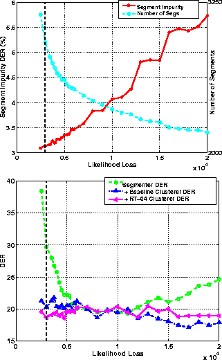
Figure 2: Effect of changing the likelihood threshold in the final stage of the segmenter. Results show the segment impurity
and number of segments, the DER of the segmenter output and the DER of the
baseline and RT-04 clusterers.
Results of varying the silence stripping threshold are given
in Table 4. The value of 1s was used as
the silence threshold since this gave the lowest sum of
missed and false alarm speech, and the lowest segment impurity.
It also gave the lowest segmenter DER.
| Silence Threshold | Dataset | Segment-Purity MS/FA/SPE/SI @ NumSeg |
Segmenter DER |
| 0.5s | didev03 | 1.8/0.8/1.0/3.57 @ 1348 | 28.9 |
| eval03 | 2.0/0.2/0.9/3.05 @ 1229 | 34.8 | |
| sttdev04 | 6.8/0.1/0.9/7.83 @ 1359 | 34.8 | |
| dev04f2 | 3.3/0.5/0.6/4.37 @ 1254 | 47.5 | |
| ALL | 3.62/0.39/0.85/4.86 @ 5190 | 36.1 | |
| 1s | didev03 | 0.6/1.6/1.0/3.21 @ 814 | 28.0 |
| eval03 | 0.6/0.8/0.9/2.21 @ 735 | 31.3 | |
| sttdev04 | 2.1/0.3/0.9/3.27 @ 814 | 30.0 | |
| dev04f2 | 1.5/1.9/0.6/3.99 @ 642 | 40.2 | |
| ALL | 1.22/1.08/0.85/3.15 @ 3005 | 32.0 | |
| 2s | didev03 | 0.2/2.6/1.1/3.93 @ 813 | 29.8 |
| eval03 | 0.4/1.8/1.0/3.14 @ 770 | 32.4 | |
| sttdev04 | 1.1/0.8/1.0/2.94 @ 804 | 31.9 | |
| dev04f2 | 1.3/3.8/0.7/5.73 @ 658 | 38.2 | |
| ALL | 0.77/2.12/0.94/3.83 @ 3045 | 32.9 |
Empty segments after the P1 stage of the ASR system are also
discarded before the final clustering stage. The effect on
the miss, false alarm and segment impurity rates is
given in Table 5. The number of segments
over the 4 datasets is reduced by 3% with no effect on segment purity.
| Stage | Dataset | Segment-Purity MS/FA/SPE/SI@ NumSeg | |
| before P1 ASR |
didev03 | 0.6/1.6/1.0/3.21 @ 814 | |
| eval03 | 0.6/0.8/0.9/2.21 @ 735 | ||
| sttdev04 | 2.1/0.3/0.9/3.27 @ 814 | ||
| dev04f2 | 1.5/1.9/0.6/3.99 @ 642 | ||
| ALL | 1.22/1.08/0.85/3.15 @ 3005 | ||
| after P1 ASR |
didev03 | 0.6/1.6/1.0/3.16 @ 790 | |
| eval03 | 0.6/0.7/0.9/2.17 @ 706 | ||
| sttdev04 | 2.2/0.3/0.9/3.36 @ 786 | ||
| dev04f2 | 1.5/1.8/0.6/3.93 @ 632 | ||
| ALL | 1.26/1.03/0.85/3.14 @ 2914 | ||
An experiment was therefore carried out into ways of sorting the
segments before clustering. Two methods of allocating the cluster
labels to the groups of segments from the segmenter were made.
The first assigned the cluster labels (bandwidth
and gender dependently) in ascending order using the first time of
each cluster to decide the ordering. The second was similar but
used the mid-time of each cluster to determine the ordering.
The segments were then sorted by this new cluster-id ( and by start time in the
case of ties) before clustering - thus ensuring that segments
assigned the same cluster-id in the segmenter would be more likely to be
initialised together in the clustering stage.
Contrast runs with no sorting or with purely time-based sorting were
also run. The results are given in Table 6.
| sorting | didev03 | eval03 | sttdev04 | dev04f2 | ALL |
| none | 18.0 | 15.9 | 21.2 | 26.9 | 20.4 |
| time | 17.5 | 16.7 | 21.5 | 25.7 | 20.2 |
| spkr-start | 17.5 | 17.9 | 22.6 | 17.5 | 19.0 |
| spkr-mid | 14.0 | 15.2 | 22.2 | 23.5 | 18.7 |
| bandwidth dependent clustering | |||||
| none | 18.3 | 18.6 | 22.4 | 26.9 | 21.4 |
| time | 18.5 | 15.8 | 20.6 | 25.7 | 20.0 |
| spkr-start | 19.4 | 17.9 | 21.3 | 20.0 | 19.7 |
| spkr-mid | 16.7 | 16.2 | 23.5 | 23.5 | 20.0 |
| bandwidth independent clustering | |||||
Although the improvements are not consistent across the datasets,
the average DER across all 24 development shows is reduced from
20.4% to 18.7% by sorting the segments by the re-assigned
segmenter cluster-id and then time, before clustering. This was used
for all further experiments. It is a little disturbing to note some of
the variation in DER from making these changes to the initialisation.
The dev04f2 data set in particular changes from 17.5 to 23.5%
just by re-allocating the initial cluster-id from its midpoint instead
of its first occurrence in the show.
Table 6 also gives results for bandwidth independent clustering. This performed worse than the bandwidth dependent case, showing that automatically detected bandwidth information can be useful in distinguishing speakers.
| Coefficients | didev03 | eval03 | sttdev04 | dev04f2 | ALL | |||
| BASE | c0 | E | Z | |||||
| PLP | - | - | - | 20.3 | 17.1 | 22.5 | 18.7 | 19.8 |
| PLP | Y | - | - | 14.0 | 15.2 | 22.2 | 23.5 | 18.7 |
| PLP | - | Y | - | 15.3 | 17.0 | 22.1 | 21.3 | 19.0 |
| PLP | Y | Y | - | 18.0 | 16.8 | 23.3 | 22.4 | 20.2 |
| PLP | Y | - | Y | 25.4 | 19.3 | 27.9 | 24.1 | 24.3 |
| MFCC | Y | - | - | 17.9 | 18.6 | 22.1 | 27.2 | 21.3 |
| MFCC | - | Y | - | 16.2 | 15.8 | 21.5 | 27.0 | 20.0 |
| MFCC | Y | Y | - | 19.7 | 19.3 | 23.5 | 27.4 | 22.4 |
| MFCC | - | Y | Y | 23.3 | 16.7 | 28.9 | 22.4 | 23.1 |
The results show that performing cepstral mean subtraction considerably degrades performance, showing that the mean information is helping distinguish speakers. However adding both c0 and the log energy did not help improve performance. The best coding with MFCCs included the log energy but this did not perform as well as the PLP coding. The best performance overall was obtained with PLP and c0 (the standard set up) but removing the c0 coefficient improved performance on the dev04f2 data by almost 5% absolute. Further investigation showed that the shows which gained most from removing the c0 coefficient often seemed to have a low mean value for the c0 coefficient over the show. Therefore an investigation was made to see if there was a feature of the c0 coding which might help predict whether the c0 coefficient should be used in clustering for optimal performance.
| Property | Correlation |
| stddev(segmean) | -0.0295 |
| mean(segmean)/stddev(segmean) | 0.0995 |
| stddev(segmean)/mean(segmean) | -0.2223 |
| mean(segmean) | 0.4223 |
| mean(show) | 0.4560 |
The correlation coefficients show that the most correlated feature
is the mean value of the c0 coefficient across the whole show
after segmentation, with a correlation of 0.456. Figure 3
shows a scatter plot of the mean c0 value against the difference
in DER when including c0 and the mean DER across all 24 development
shows when the clustering uses c0 if and only if the mean c0 value
after segmentation is above a certain threshold. The breakdown in
results over the different datasets is given in Table 9.
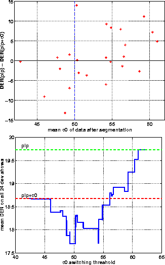
Figure 3: (a) Scatter plot showing the difference in DER when omitting the c0 coefficient against the mean c0 value for each development show. (b) Mean DER across all 24 development shows when only including c0 in clustering if the mean value is above a critical threshold.
| c0thresh | didev03 | eval03 | sttdev04 | dev04f2 | ALL |
| 0 (PLP+c0) | 14.0 | 15.2 | 22.2 | 23.5 | 18.7 |
| 48 | 14.0 | 15.2 | 22.2 | 22.3 | 18.5 |
| 49 | 14.0 | 15.2 | 21.8 | 20.3 | 17.9 |
| 50 | 14.0 | 15.5 | 21.8 | 19.2 | 17.7 |
| 51 | 16.6 | 15.5 | 21.2 | 19.2 | 18.2 |
| 52 | 16.6 | 15.5 | 21.2 | 18.7 | 18.1 |
| 54 | 16.6 | 15.5 | 21.2 | 18.7 | 18.1 |
| 56 | 18.6 | 15.5 | 21.2 | 18.7 | 18.6 |
| 100 (PLP) | 20.3 | 17.1 | 22.5 | 18.7 | 19.8 |
The results show the mean DER over the 24 shows can be reduced from 18.7% to 17.7%, with the DER on the dev04f2 dataset (closest in epoch to the eval04f data) reduced from 23.5% to 19.2% if this method is used with a threshold of 50. However, there was some concern that this may not hold across new datasets, so the c0-switching was implemented as a contrast run for the RT-04 evaluation, the primary run using c0 in the clustering stage for all cases.
The final clustering stage is run as before, but the preceding
clustering stages can be run differently if required. For example,
producing many clusters would minimise the risk of segments being falsely
combined, whereas producing fewer clusters than normal and
relying on the temporal adjacency criterion to restrict false
combinations might also be justified.
The results for α of 7.25 (optimal), 5 (conservative) and
10 (overclustered) for the non-final iteration are presented
in Table 10 and
the segment purity for the case of using the optimal α = 7.25 throughout
is given in Table 11.
| non-final α | iterations | eval03 | didev03 | sttdev04 | dev04f2 | OVERALL |
| - | 0 | 63.3 | 59.7 | 62.4 | 67.5 | 63.1 @ 2914 |
| - | 1 | 15.2 | 14.0 | 22.2 | 23.5 | 18.7 @ 2629 |
| 7.25 | 2 | 14.9 | 15.9 | 22.6 | 23.6 | 19.3 @ 2587 |
| 7.25 | 3 | 15.6 | 14.8 | 22.3 | 23.7 | 19.1 @ 2570 |
| 7.25 | 10 | 15.6 | 15.0 | 22.0 | 23.7 | 19.1 @ 2565 |
| 5 | 2 | 15.3 | 15.9 | 23.1 | 24.3 | 19.7 @ 2609 |
| 5 | 3 | 16.7 | 17.3 | 24.3 | 28.9 | 21.7 @ 2616 |
| 5 | 10 | 16.4 | 18.6 | 23.6 | 28.1 | 21.6 @ 2621 |
| 10 | 2 | 15.0 | 17.5 | 21.6 | 23.1 | 19.3 @ 2540 |
| 10 | 3 | 16.9 | 17.8 | 24.6 | 24.0 | 20.9 @ 2521 |
| 10 | 10 | 19.9 | 21.3 | 25.3 | 22.9 | 22.4 @ 2515 |
| iter | didev03 | eval03 | sttdev04 | dev04f2 | ALL |
| 0 | 1.0 @ 790 | 0.9 @ 706 | 0.9 @ 786 | 0.6 @ 632 | 0.85 @ 2914 |
| 1 | 1.6 @ 714 | 0.9 @ 644 | 1.9 @ 702 | 1.2 @ 569 | 1.43 @ 2629 |
| 2 | 2.1 @ 694 | 1.0 @ 638 | 2.0 @ 695 | 1.2 @ 560 | 1.59 @ 2587 |
| 3 | 2.2 @ 686 | 1.4 @ 635 | 2.2 @ 691 | 1.2 @ 558 | 1.80 @ 2570 |
| 10 | 2.3 @ 681 | 1.4 @ 635 | 2.2 @ 691 | 1.2 @ 558 | 1.82 @ 2565 |
The results show that this technique did not help improve performance overall, producing a increase in segment impurity and corresponding increase in final DER even after only one extra iteration, for all datasets except the eval03 data.
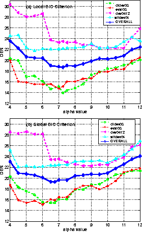
Figure 5: Effect of changing the α value in the clustering when using the full correlation matrix with static only PLP coefficients. (a) uses the 'local' whilst (b) uses the 'global' formulation.
| Coding | Segmentation | Clustering | DER main | DER c0switch |
| RT-03s | RT-03s | RT-03s | 36.33 | - |
| RT-03s | RT-03s | RT-04 | 27.90 | 24.45 |
| RT-03s | RT-04 | RT-04 | 22.48 | 22.35 |
| ¹ RT-04 | RT-04 | RT-04 | 23.86 | 24.12 |
The contrast run which included the c0-switching did perform better
when using the RT-03s segmentation (24.5% instead of 27.9%) but made
little difference when used with the RT-04 segmenter.
An experiment was run to see the effect of using different criteria to pick the likelihood threshold and clustering strategy on the dev data. Three different strategies were tried namely (a) just use the segmenter output which gave the best segmenter DER; (b) use the clusterer output which gave best performance across all the dev data; and (c) use the clusterer output which gave best performance on the dev04f2 data, since this was closest in epoch to the eval04f data. The results are given in Table 13 using the RT-03s PLP coding.
| likelihood thresh | post-ASR Segment Impurity |
Segmenter DER | Baseline Clusterer DER |
RT-04 Clusterer DER |
| 3000 | 0.4/1.1/1.2/2.69 @ 1383 | 35.15 | 22.03 | 22.48(e) |
| 11000 | 0.4/1.1/2.2/3.73 @ 1063 | 18.72(a1) | 22.90 | 21.02 |
| 16000 | 0.4/1.1/3.8/5.35 @ 987 | 21.17 | 20.50(c) | 22.18 |
| 17000 | 0.4/1.1/3.9/5.44 @ 988 | 22.05 | 22.06(b) | 21.44 |
| ¹ 2600 | 0.4/1.1/3.5/5.05 @ 979 | 18.12(a2) | 21.82 | 23.49 |
The results show that the eval04f DER could have been reduced by changing the strategy used to finalise the system on the dev data, the best performance being 18.1% when using the segmenter output directly (with no differentials in the feature vector in the full-covariance stage).
This work was supported by DARPA grant MDA972-02-1-0013. The paper does not necessarily reflect the position or the policy of the US Government and no official endorsement should be inferred.