|
|
|||
 |
Department of Engineering |
| University of Cambridge > Engineering Department > Machine Intelligence Lab > Medical Imaging Group |
Ultrasound images in medicine usually display the amount of sound reflected back from anatomy (B,C or M-mode scans) or the flow in a vessel (Colour or Power Doppler). The former usually displayed as a grey-scale image, and the latter as a grey-scale image with a red-yellow or blue image superimposed onto it.
However, this is not the only anatomical information which can be displayed from an ultrasound signal. This page details some on-going research into two other sorts of ultrasound displays. The first is ultrasound attenuation, i.e. the amount of sound absorbed by the tissue rather than reflected. The second is strain (often referred to as elastographic imaging), which shows how soft or hard the anatomy is.
Both the techniques described below are very fast (less than one second on a normal PC). Strain imaging is already undergoing clinical evaluation, whereas attenuation imaging only currently works well on in vitro data.
Conventional ultrasound images (B-scans) display the amount of reflected sound received back at the ultrasound probe. However, this sound is attenuated (or reduced) as it passes through the anatomy. The amount of reduction depends on the anatomy which the sound passes through. So what you see at one location in a B-scan will depend not only on the reflection at that point, but also on the attenuation in the anatomy above that point.
Attenuation could be an important diagnostic material parameter, but failure to adjust for variations in attenuation also causes several of the artefacts in B-scans. So called 'shadowing' (dark vertical strips below bright regions) and 'enhancement' (light vertical strips below dark regions) are both caused by varying attenuation. So if we can measure attenuation we could 'correct' conventional B-scans as well as displaying it in it's own right.
 |
 |
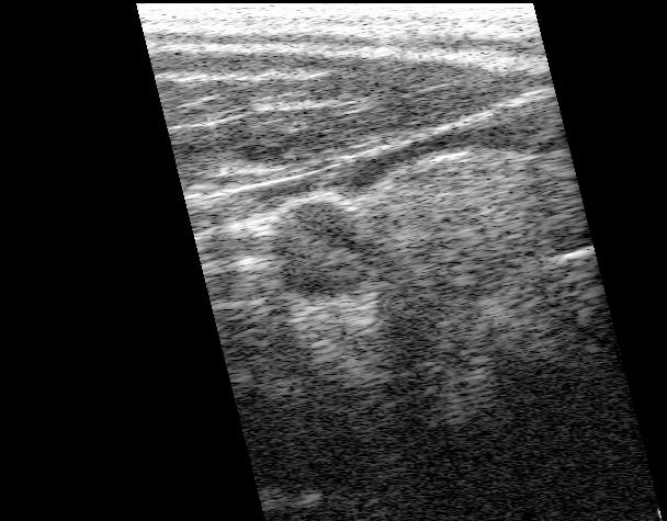 |
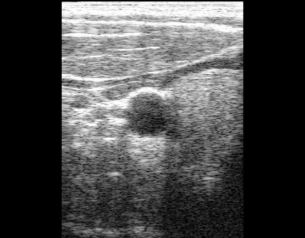
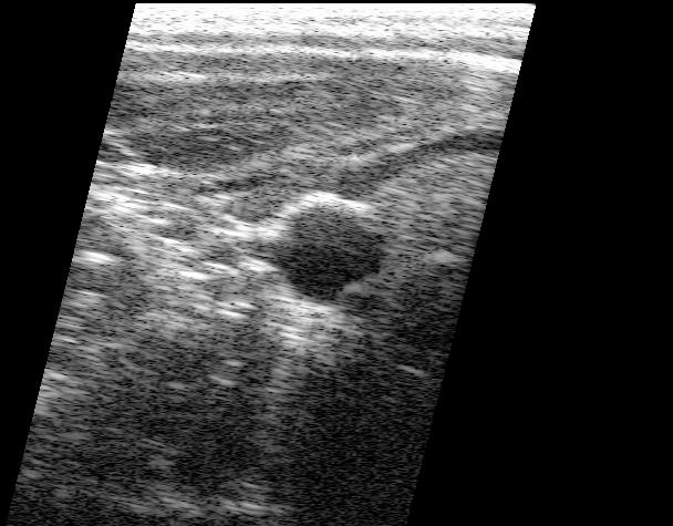
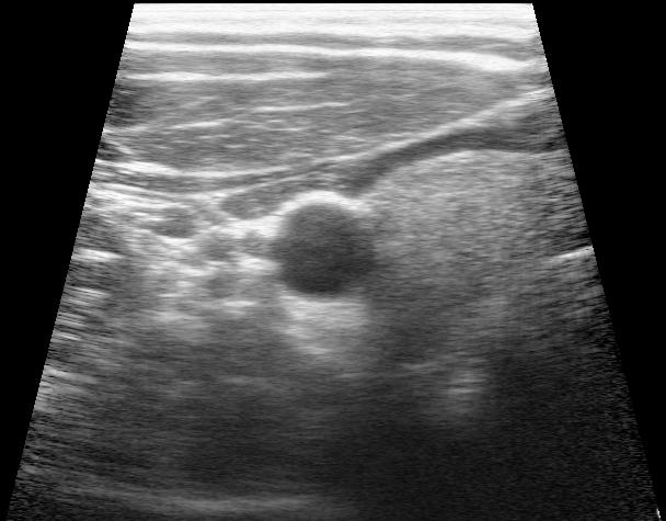
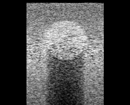
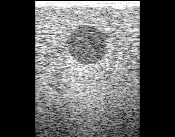
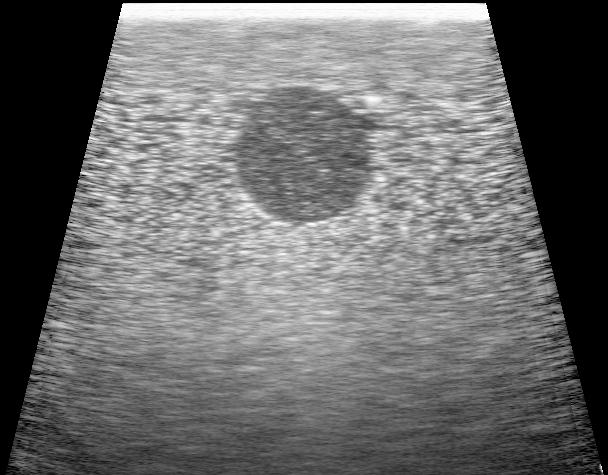
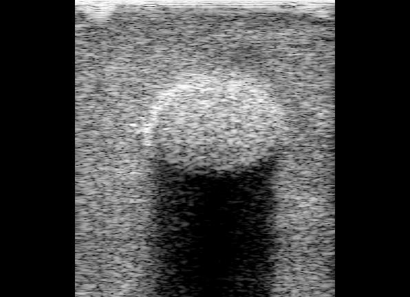
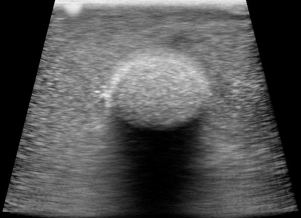
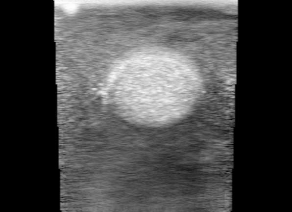
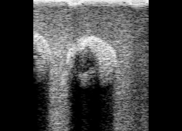
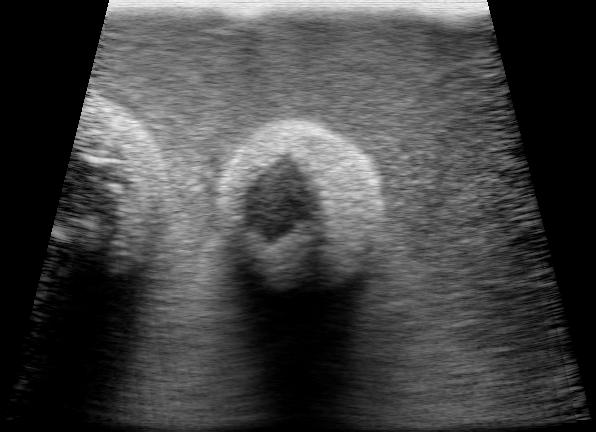
| (a) Normal B-scan | (b) Steered to -14 deg | (c) Steered to +14 deg |
Figure 1. Ultrasound Beam-steering. (a) the beam is normally steered straight down, but can be steered at slight angles (b) and (c) by changing the transmit and receive delays.
|
 |
 |
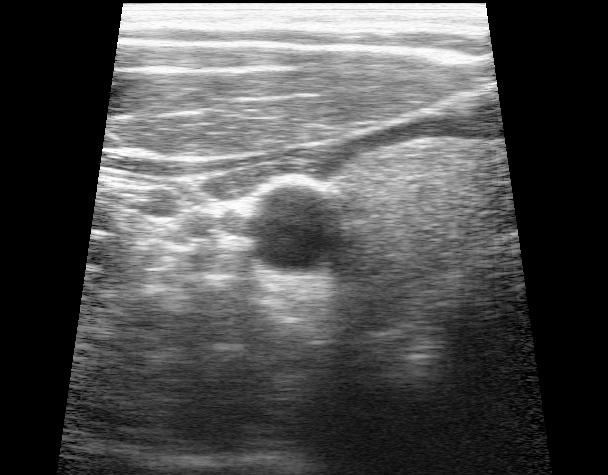
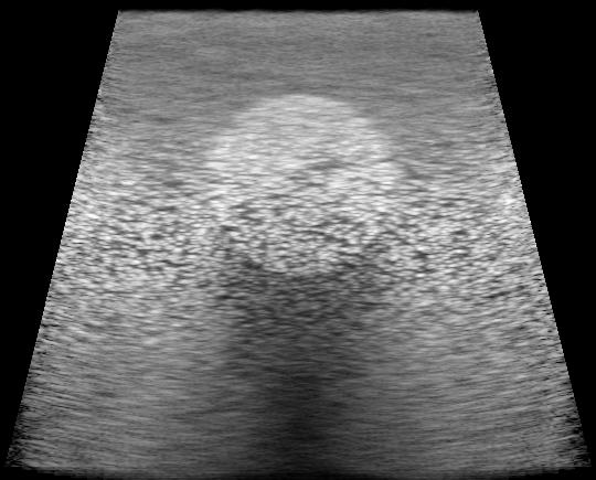
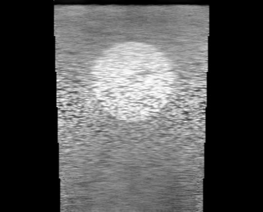
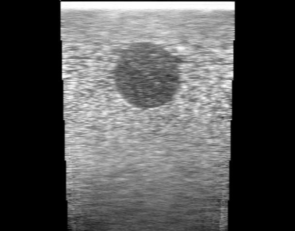
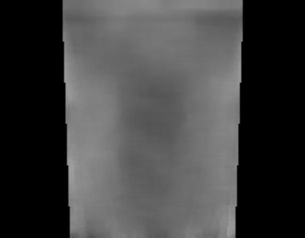
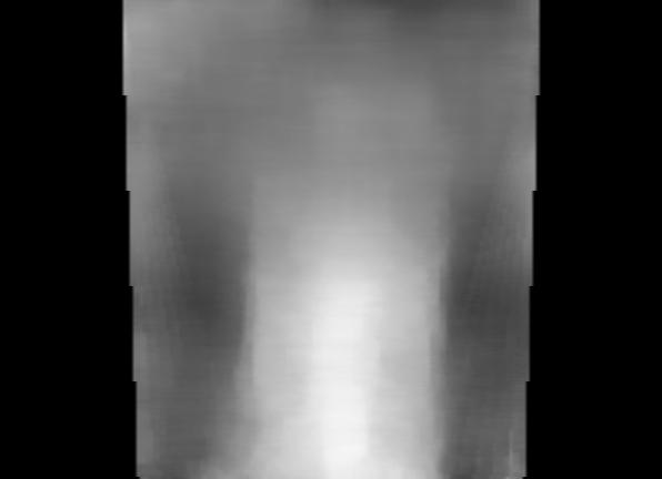
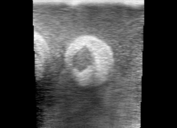
| (a) Normal B-scan | (b) Compounded -6 to 6 deg | (c) Compounded -14 to 14 deg |
Figure 2. Compounding. (a) individual B-scans can be averaged to produce compounded images (b) and (c) with better signal-to-noise.
One way of reducing shadowing is to display compounded images by steering the ultrasound beam, as in Figure 1. Compounding improves the quality of the ultrasound data (Figure 2) and reduces the shadows, but it does not eliminate them.
Instead of averaging scans from different directions, we can process them to calculate the attenuation in the image. Having done so, we can then display a 'corrected' B-scan, and also the attenuation itself. Examples of this are shown below. At the moment, this only works well in in vitro data - methods for improving performance in in vivo data are an active research topic.
 |
 |
 |
 |
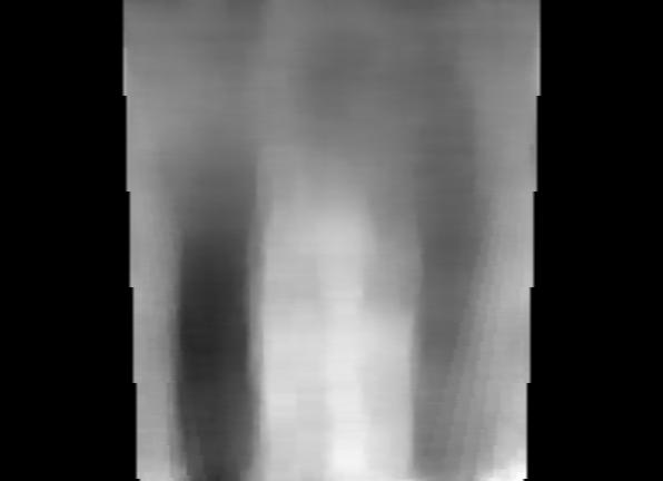
| (a) B-scan | (b) Compounded | (c) Corrected | (d) Attenuation |
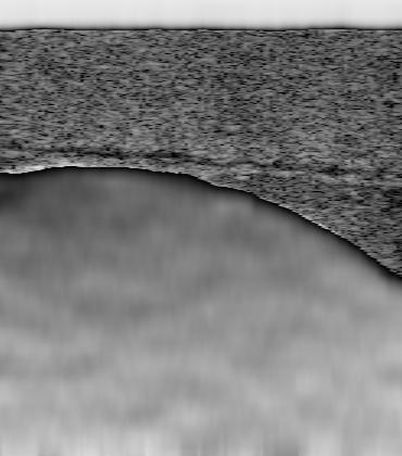
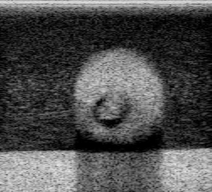
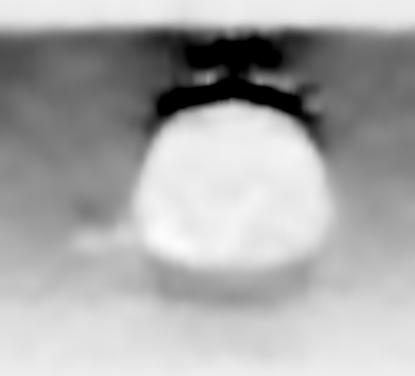
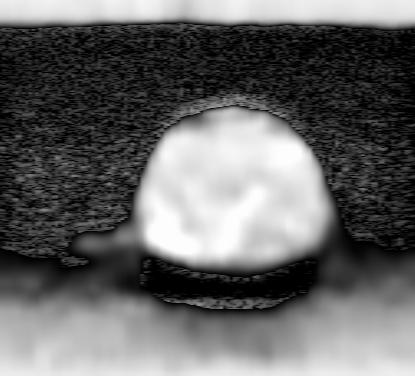
Figure 3. Correction in simulated data. (a) a conventional B-scan, (b) compounding improves SNR but does not remove the shadow, (c) corrected for attenuation, (d) the cumulative attenuation.
 |
 |
 |
 |
| (a) B-scan | (b) Compounded | (c) Corrected | (d) Attenuation |
Figure 4. Correction in in vitro data. (a) a conventional B-scan, (b) compounding improves SNR but does not remove the shadow, (c) corrected for attenuation, (d) the cumulative attenuation.
 |
 |
 |
 |
| (a) B-scan | (b) Compounded | (c) Corrected | (d) Attenuation |
Figure 5. Correction in in vitro data. (a) a conventional B-scan, (b) compounding improves SNR but does not remove the shadow, (c) corrected for attenuation, (d) the cumulative attenuation.
 |
 |
 |
 |
| (a) B-scan | (b) Compounded | (c) Corrected | (d) Attenuation |
Figure 6. Correction in in vitro data. (a) a conventional B-scan, (b) compounding improves SNR but does not remove the shadow, (c) corrected for attenuation, (d) the cumulative attenuation.
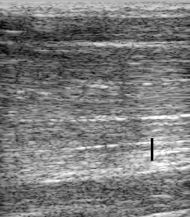
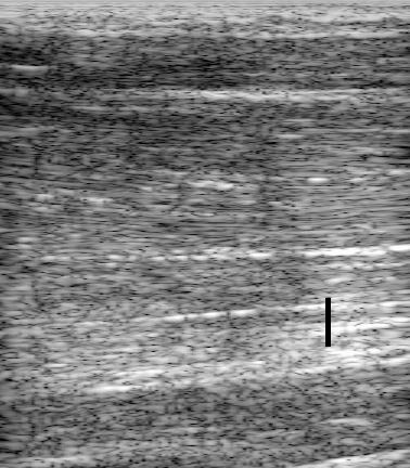
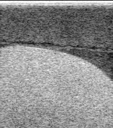
It is also possible to deduce relative anatomical stiffness by looking at ultrasound data. First we take two B-scans of the same anatomy, but one with a very slightly different probe contact pressure. The contact pressure only has to vary by a very small amount, for instance compare the two B-scans in Figure 7 (a) and (b). We then look at small sections of the original radio-frequency data (on which the B-scan is based), like the black strips in the figure. We can then compare the exact locations of these sections in both B-scans using a very accurate algorithm. This gives us an estimate of relative vertical displacement between the two B-scans, as in Figure 7 (c).
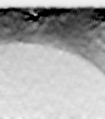
We then look at the gradient of this displacement - this shows the strain at this location in the image. An image of strain (Figure 7 (d)) reveals the relative stiffness of the anatomy. This potentially has significant clinical impact, particularly in spotting small tumours which are often stiffer than the surrounding tissue.
 |
 |
 |
 |
| (a) B-scan | (b) very slightly deformed | (c) relative displacement | (d) strain |
Figure 7. In vivo strain estimation. Two B-scans are compared with very slight relative deformation (<1%), due to probe contact pressure (a) and (b). The relative displacement is estimated (c) by comparing lots of small windows of data e.g. those shown in black. (d) the gradient of displacement gives strain.
The following are several examples of conventional B-scans and corresponding strain images.
 |
 |
 |
| (a) B-scan | (b) strain | (c) overlay |
Figure 8. In vitro strain estimation.
 |
 |
 |
| (a) B-scan | (b) strain | (c) overlay |
Figure 9. In vitro strain estimation.
 |
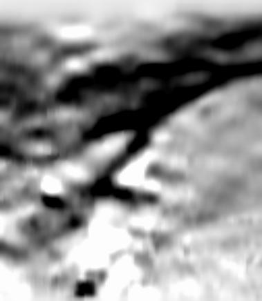 |
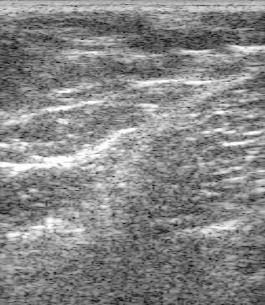
| (a) B-scan | (b) strain |
Figure 10. In vivo strain estimation.
| | Search | CUED | Cambridge University | |
|
©
2005 Cambridge University Engineering Dept
and Graham Treece
.
Information provided by gmt11 |